Welcome to ResMicroDb
Welcome to ResMicroDb1. Introduction1.1 Overview of ResMicroDb1.2 Citation1.3 Contact us1.4 Licenses2. Materials and Methods2.1 Data Collection2.1.1 Literature search2.1.2 Raw sequencing data download2.1.3 Metadata download and curation2.2 Data Processing2.2.1 Quality control and Taxonomic assignment2.2.2 Case-control Analysis2.2.2.1 Identification of microbe-disease associations (markers)2.2.2.2 Diversity Analysis2.2.3.3 Microbial Co-occurrence Network Analysis3. Database Usage3.1 Home3.2 Sample Sites3.3 Taxa3.3.1 Overview of All Taxa3.3.2 Taxa Details3.4 Phenotypes3.4.1 Overview of all phenotypes3.4.2 Phenotype details3.5 Associations/Markers3.6 Samples3.7 Projects3.7.1 Overview of all projects3.7.2 Project details3.8 Publications3.9 Microbiome Composition3.10 Sample Similarity search3.11 Cross-study Analysis3.11.1 Marker3.11.2 Diversity3.11.3 Network3.12 Statistics3.13 Download
1. Introduction
1.1 Overview of ResMicroDb
Respiratory diseases pose a major burden to global public health. Distinct anatomical sites within the human respiratory tract harbor unique resident microbial communities, which play important roles in susceptibility, clinical progression, and outcomes of both infectious and non-infectious diseases. The number of studies on the respiratory microbiome has surged recently, along with a substantial increase in data. However, there is a notable lack of a comprehensive respiratory microbiome database.
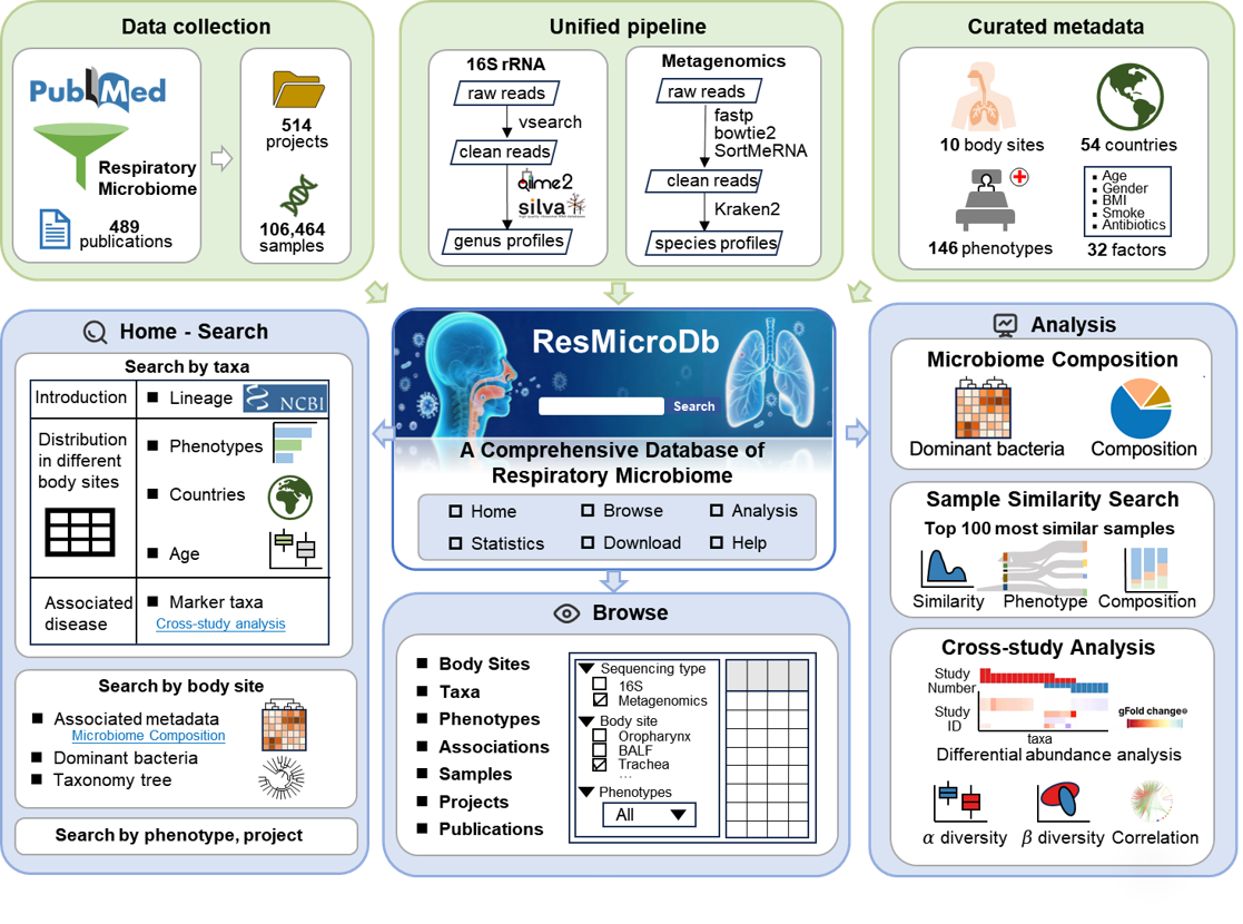
To fill this gap, we introduce ResMicroDb, a comprehensive database and analysis platform for the human respiratory microbiome. ResMicroDb integrates 106,464 samples from 489 publications and 514 projects, covering 10 sample sites and 146 phenotypes.Specifically, ResMicroDb provides the following data resources: (1) standardized microbiome profiles for all samples generated using a unified processing pipeline; (2) a total of 32 manually curated metadata factors; (3) distributions of 3,490 microbial taxa across sample sites, phenotypes, countries, and age groups; and (4) 11,908 microbe-disease associations identified from 132 case-control studies. In addition, ResMicroDb offers three online tools for further analysis: (1) Microbiome Composition: generates microbiome profiles for selected samples. (2) Sample Similarity Search: finds the most similar samples in the database to a user-provided query. (3) Cross-study Analysis: explores both shared and unique microbial characteristics across cohorts, diseases, and sample sites. Overall, this comprehensive database, along with its integrated analysis tools, will serve as a versatile and valuable resource for advancing research across a broad spectrum of respiratory microbiome studies.
1.2 Citation
Please cite: Ji X, Qian Q, Zhang H, Cai Q, Zhang K, Xiao J, Jiang X, Li M. ResMicroDb: a comprehensive database and analysis platform for the human respiratory microbiome. Nucleic Acids Res. 2025 Dec 3:gkaf1194.
1.3 Contact us
If you have any question, suggestions, or comments, please feel free to contact us via email (limk@cncb.ac.cn).
Address:
National Genomics Data Center
Beijing Institute of Genomics (China National Center for Bioinformation), Chinese Academy of Sciences
No. 104 building, No.1 Beichen West Road, Chaoyang District
1.4 Licenses
ResMicroDb is free for academic use only. For any commercial use, please contact us for commercial licensing terms.
2. Materials and Methods
2.1 Data Collection
2.1.1 Literature search
We searched the PubMed database up to January 31, 2025 using keywords “human” AND “[respiratory]” AND “microbiome”. The term “[respiratory]” was also substituted with specific respiratory site names, such as “oropharynx”, “trachea”, “lung” and others. Out of 10,586 records retrieved, we manually reviewed full text of each publication and excluded those did not focus on the respiratory microbiome or without accessible raw data. Finally, 489 publications were retained.
Search Query for Respiratory Microbiome Articles
x1((2"microbiota"[MeSH Terms] OR "microbiom*"[Title/Abstract] OR "microbiota*"[Title/Abstract]3OR "bacteriom*"[Title/Abstract]4OR "mycobiome"[MeSH Terms] OR "mycobiom*"[Title/Abstract]5OR "virome"[MeSH Terms] OR "virom*"[Title/Abstract]6OR "metagenomics"[MeSH Terms] OR "metagenome"[MeSH Terms] OR "metagenom*"[Title/Abstract]7OR "metatranscriptom*"[Title/Abstract]8OR "amplicon*"[Title/Abstract]9OR "rna, ribosomal, 16s"[MeSH Terms] OR "16s"[Title/Abstract]10OR "rna, ribosomal, 18s"[MeSH Terms] OR "18s"[Title/Abstract]11OR "shotgun*"[Title/Abstract]12OR "mNGS"[Title/Abstract]13OR "microecology"[Title/Abstract]14)15AND16(17"respiratory system"[MeSH Terms] OR "respiratory*"[Title/Abstract]18OR "respiration"[MeSH Terms] OR "respiration"[Title/Abstract]19OR "LRT"[Title/Abstract] OR "URT"[Title/Abstract]20OR "airway*"[Title/Abstract]21OR "hypopharynx"[MeSH Terms] OR "hypopharyn*"[Title/Abstract]22OR "larynx"[MeSH Terms] OR "laryn*"[Title/Abstract]23OR "nasopharynx"[MeSH Terms] OR "nasopharyn*"[Title/Abstract]24OR "oropharynx"[MeSH Terms] OR "oropharyn*"[Title/Abstract]25OR "pharynx"[MeSH Terms] OR "pharyn*"[Title/Abstract] OR "throat*"[Title/Abstract]26OR "paranasal sinuses"[MeSH Terms] OR "sinus*"[Title/Abstract] OR "paranasal"[Title/Abstract]27OR "trachea"[MeSH Terms] OR "trachea*"[Title/Abstract]28OR "bronchi"[MeSH Terms] OR "bronchoscopy"[MeSH Terms] OR "bronch*"[Title/Abstract]29OR "alveol*"[Title/Abstract]30OR "lung"[MeSH Terms] OR "lung*"[Title/Abstract] OR "pulmo*"[Title/Abstract]31OR "sputum"[MeSH Terms] OR "sputum*"[Title/Abstract] OR "sputa"[Title/Abstract]32OR "endotrachea*"[Title/Abstract]33OR "bronchi"[MeSH Terms] OR "bronchoscopy"[MeSH Terms] OR "bronch*"[Title/Abstract]34OR "bronchoalveolar lavage fluid"[MeSH Terms] OR "bronchoalveolar lavage fluid"[Title/Abstract]35OR ("bronchoalveolar"[Title/Abstract] AND "lavage"[Title/Abstract] AND "fluid"[Title/Abstract])36))37AND38(humans[Filter] AND (2010/1/1:2025/1/31[pdat]))
2.1.2 Raw sequencing data download
We downloaded raw microbiome sequencing data in FASTQ format from NCBI SRA, EBI ENA, and NGDC GSA.
parallel-fastq-dump: download NCBI SRA data
xxxxxxxxxx11parallel-fastq-dump -s ${run accession} --gzip --skip-technical --split-3enaBrowserTools: download EBI ENA data
xxxxxxxxxx11enaDataGet -s ${run accession} -f fastqxxxxxxxxxx11ascp -P33001 -i ${aspera_key_file} -QT -l100m -k1 -d ${run accession}2.1.3 Metadata download and curation
To ensure maximal completeness and accuracy of the metadata, we performed manual curation and standardization on most metadata obtained from the BioSample database. The curation process involved cross-referencing the original research articles associated with each BioProject, verifying the consistency between the published data, supplementary materials, and the corresponding BioSample metadata. Standardization of metadata of all samples are done based on the structured curation model below.
Structured Metadata Curation Model
| Items | Description | Value (Grey letters: prefix of accession numbers) |
| Basic information | ||
| Run | Accession number of each sample from data resource | SRR, ERR, DRR or CRR |
| Project ID | Accession number of each BioProject from data resource | PRJNA, PRJEB, PRJDB or PRJCA (Some projects do not have an Accession number, we use their SRAStudy accession number for replacement.) |
| BioSample | Accession number of each Biosample in data resource | SAMN, SAMEA, SAMD or SAMC |
| PMID | Publication in which the sampe is described | PubMed ID |
| Sequencing Strategy | ||
| Sequencing Type | Controlled vocabulary | 16S, Metagenomics, Metatranscriptomics |
| Library Layout | Controlled vocabulary | SINGLE or PAIRED |
| Platform | Controlled vocabulary | ILLUMINA, LS454, BGISEQ, ION_TORRENT |
| Model | Controlled vocabulary | Illumina MiSeq, Illumina NovaSeq 6000, Illumina HiSeq 2500, etc |
| 16S Region | Controlled vocabulary | V4, V3, V1-V2, V1-V3, V3-V4, V3-V5, etc |
| Biological Condition | ||
| Phenotype | Controlled vocabulary | To establish a standardized framework for disease names and definitions, terms or identifiers from multiple ontologies, including Experimental Factor Ontology (EFO) (Main source)、Mondo Disease Ontology (MONDO)、NCI Thesaurus OBO Edition (NCIT)、SNOMED CT (International Edition) (SNOMED)、 Human Disease Ontology (DOID)、 Human Phenotype Ontology (HP)、TOXic Process Ontology (TXPO) and Ontology for MIRNA Target (OMIT). |
| Disease Stage | The disease stage of samples | Conclusion term |
| Complication | The complication of samples | Conclusion term |
| Smoking | Controlled vocabulary | Non-smoker, Smoker, Ex-Smoker |
| Recent Antibiotic Use | Controlled vocabulary | Yes, No |
| Antibiotics Used | The antibiotics used for the samples | Conclusion term |
| Sample Characteristic | ||
| Sample Site | Controlled vocabulary | Nasal, Nasopharynx, Oropharynx, Pharynx, Throat, Sputum, Trachea, Bronchus, BALF, Lung Tissue |
| Sample Type | Sample Site recorded in the original publication/study | Conclusion term |
| Sex | Controlled vocabulary | Male, Female |
| Age | Statistical data | The age of samples, recorded as either a specific value or an interval |
| Age Group | Controlled vocabulary | 0-3, 3-18, 18-35, 35-45, 45-60, 60-75, 75+ |
| BMI | Statistical data | The BMI of samples, recorded as either a specific value or an interval |
| Patient ID | A unique identifier for each patient as recorded in the original publication/study | Conclusion term |
| Time Point | The time point at which the sample was collected | Conclusion term |
| #Reads | Statistical data | The number of reads in the sample |
| Shannon | Statistical data | Shannon-Wiener index, a measure of taxa diversity in a community |
| Chao1 | Statistical data | Chao1 index, an estimator of taxa richness in a community |
| Observed | Statistical data | The observed number of unique taxa within a community |
| Geographic Location | ||
| Continent | Controlled vocabulary | Europe, North America, Asia, Africa, Oceania, South America |
| Country | Controlled vocabulary | United States, China, Netherlands, United Kingdom, etc |
| Location | Controlled vocabulary | Bilthoven, Copenhagen, New York, Shenzhen, etc |
| Latitude | The geographic latitude coordinate | Generated by geocoding the 'Country' and 'Location' fields using Google Maps |
| Longitude | The geographic longitude coordinate | Generated by geocoding the 'Country' and 'Location' fields using Google Maps |
2.2 Data Processing
2.2.1 Quality control and Taxonomic assignment
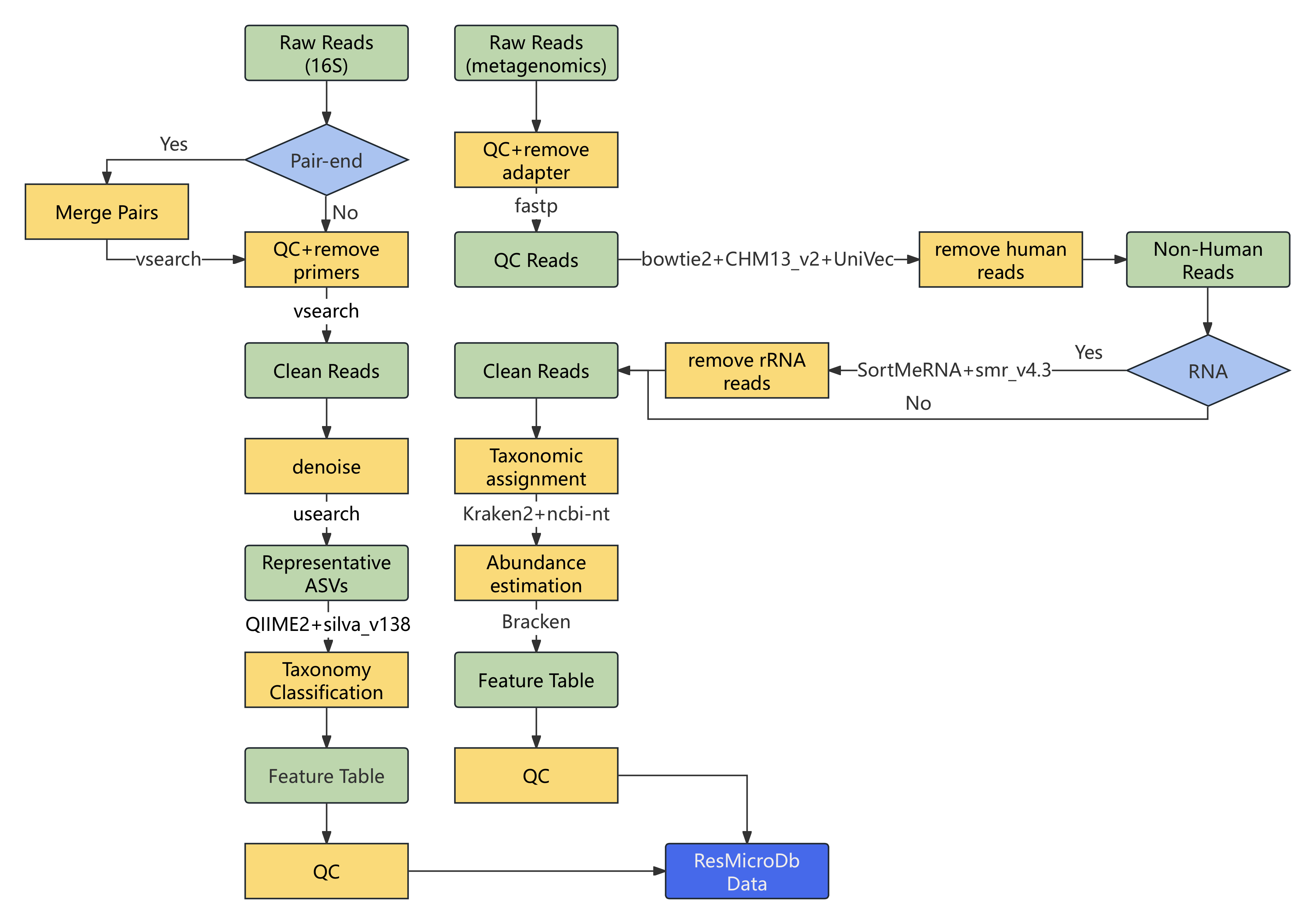
For 16S rRNA gene sequencing data (Figure 2, left), we performed: (1) Read merging and quality control using VSEARCH; (2) Denoising and chimera removal to generate Amplicon Sequence Variants (ASVs) using USEARCH; (3) Taxonomy classification using the QIIME2 feature-classifier plugin and the SILVA ribosomal RNA database (v138).
For metagenomic and metatranscriptomic sequencing data (Figure 2, right), we performed: (1) Quality control using fastp; (2) Host (T2T-CHM13) and contaminant (UniVec) sequences removal using Bowtie2; (3) Ribosomal RNA removal using SortMeRNA; (4) Taxonomic classification using Kraken2 with a custom database (NCBI nucleotide sequences for bacteria/archaea/viruses/fungi plus T2T-CHM13); (5) Abundance estimation using Bracken at the species level.
2.2.2 Case-control Analysis
For the 132 case-control studies collected, we performed microbial biomarker identification, biodiversity analysis, and co-occurrence network construction for each individual study to systematically compare microbiome differences between the disease and control groups. Additionally, Cross-study Analysis was conducted to identify consistent associations across studies.
2.2.2.1 Identification of microbe-disease associations (markers)
Marker taxa are genera or species significantly differentially abundant between case and control groups (absolute gFold Change > 0.1 and BH-adjusted p-value <= 0.2) by differential abundance analysis (DAA).
We employed multiple DAA methods to provide users with diverse options. These methods include the Wilcoxon rank-sum test, fastANCOM, ALDEx2, MaAsLin2, and ZicoSeq, with MaAsLin2 set as the default method.
For effect size quantification, we employed generalized fold change (gFold Change). Generalized fold change is the mean of the differences between two distributions at several quantiles and can therefore resolve differences in low-prevalence taxa. The formula is as follows:
Where:
Q: Set of quantiles, {0.1,0.2,…,0.9}
ϵ: Pseudocount,1e-6
n: Number of quantiles evaluated (n = 10)
2.2.2.2 Diversity Analysis
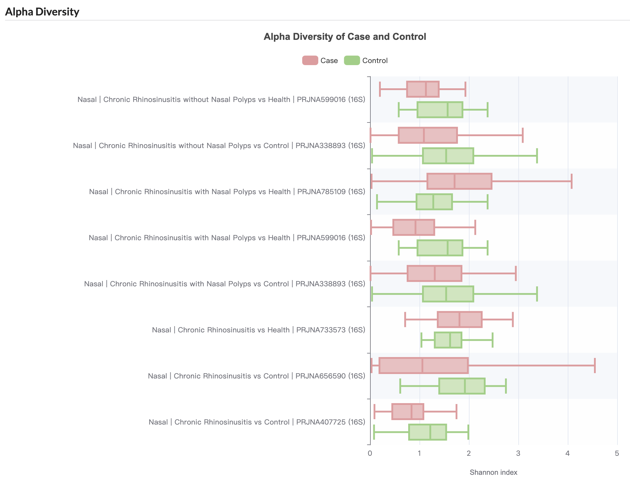
Alpha diversity was assessed using the Shannon index, and group comparisons were made using the Wilcoxon rank-sum test.
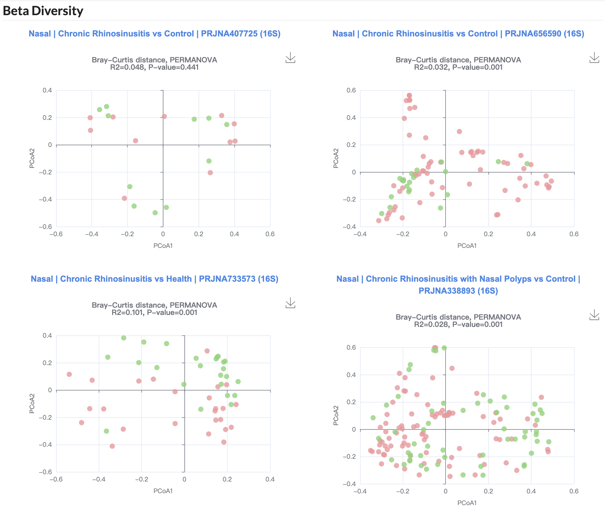
Beta diversity was evaluated through principal coordinates analysis (PCoA) based on Bray-Curtis distance, with group differences tested using permutational multivariate analysis of variance (PERMANOVA).
2.2.3.3 Microbial Co-occurrence Network Analysis
We constructed microbial co-occurrence networks for disease and control groups separately using the NetCoMi package, with microbial interactions calculated by the SparCC method and network differences between groups compared using the netCompare function.
Network comparisons were performed across various properties of the whole network, the largest connected component, and individual nodes.
Network properties
| Network feature | Description |
|---|---|
| Number of components | Number of connected components. Since a single node is connected to itself by the trivial path, each single node is a component. |
| Clustering coefficient | A measure of the network's "cliquishness", defined as the arithmetic mean of the local clustering coefficient defined by Barrat et al. It quantifies the degree to which nodes tend to cluster together. |
| Positive edge percentage | Percentage of edges with positive estimated association of the total number of edges. It reflects the balance of cooperative versus competitive interactions. |
| Edge density | The density of a graph is the ratio of the actual number of edges and the largest possible number of edges in the graph, assuming that no multi-edges are present. It measures the overall connectivity saturation of the network. |
| Natural connectivity | The natural connectivity of a graph is a useful robustness measure of complex networks, corresponding to the average eigenvalue of the adjacency matrix. |
| Relative LCC size | The proportion of nodes within the LCC relative to the total number of nodes in the entire network. |
| Clustering coefficient | A measure of the cliquishness or degree to which nodes cluster together, calculated for the LCC. |
| Positive edge percentage | The proportion of positive edges relative to the total number of edges, calculated for the LCC. |
| Edge density | The ratio of actual edges to the maximum possible number of edges, calculated for the LCC. |
| Natural connectivity | A measure of structural robustness based on path redundancy, calculated for the LCC. |
| Vertex connectivity | The minimum number of vertices that must be removed to disconnect the LCC. It measures vulnerability to node loss. |
| Edge connectivity | The minimum number of edges that must be removed to disconnect the LCC. It measures vulnerability to link disruption. |
| Average dissimilarity | The mean of the dissimilarity values (e.g., 1 - correlation) across all edges in the LCC. |
| Average path length | Computed as the mean of shortest paths in the LCC. The av. path length of an empty network is 1. |
| Degree centrality | Degree centrality refers to a measure in network analysis that quantifies the number of connections a node has. It is calculated based on the count of social connections (edges) a node possesses, with higher values indicating a more central position within the network. |
| Betweenness centrality | A measure of how often a node lies on the shortest paths between other nodes. It identifies crucial "bridges" or bottlenecks. |
| Closeness centrality | A measure of how close a node is to all other reachable nodes. It quantifies a node's overall accessibility in a network by measuring the normalized inverse of its total shortest-path distance to all other reachable nodes. |
| Eigenvector centrality | A measure of a node's influence, where connections to other highly influential nodes contribute more to its score. |
3. Database Usage
3.1 Home
The Home page provides a general overview of ResMicroDb and its main features. Users can:
Perform quick searches via the search box.
Click on icons or statistics to navigate to corresponding database sections.
3.2 Sample Sites
The Sample Sites page displays 10 respiratory sites included in ResMicroDb.
a) Associated metadata: Categorizes samples based on metadata such as "Phenotype" and "Sequencing Type." By clicking on the Microbiome Composition, users can explore detailed microbial profiles and (only available for sample sizes ≥10).
b) Dominant taxa:Shows the average relative abundance of the top 15 genera across all nasopharynx samples, healthy samples (include Control samples) and disease samples. Columns represent individual samples, with hierarchical clustering performed using the Bray-Curtis distance matrix and the Ward.D2 method.
c) Taxonomy tree:Displays the taxonomic hierarchy of the top 100 most prevalent genera in all nasopharynx samples, healthy samples (include Control samples) and disease samples. Solid dots indicate genera with a prevalence greater than 0.6, representing core taxa.
3.3 Taxa
3.3.1 Overview of All Taxa
The Taxa page displays 3,490 taxa (1,117 genus and 2,373 species) included in ResMicroDb, along with their presence across healthy (include Control samples) and disease samples, as well as the number of microbe-disease associations.
Users can click on any taxon to view detailed information. (The quick search bar on the Home page can also be used for access)
3.3.2 Taxa Details
Here we use Streptococcus as an example to show the contents of this page.
a) Introduction: Includes lineage, NCBI TaxID, description, and links to external databases such as the NCBI Taxonomic Database, Wikipedia, and BugSigDB.
b) Distribution in different sample sites: Displays the distribution of Streptococcus across different sample sites and sequencing types, showing abundance and prevalence in both healthy (include Control samples) and diseased samples. Clicking on visualizations provides comprehensive characteristics under more metadata (e.g., distribution in nasopharynx across phenotypes, countries, and age groups).
c) Marker taxon: Lists diseases associated with Streptococcus. Markers are identified on a per-project basis. (Refer to the Identification of Microbe-Disease Associations for detailed marker identification process.)
3.4 Phenotypes
3.4.1 Overview of all phenotypes
The Phenotypes page displays 146 phenotypes included in ResMicroDb, along with the number of associated samples, studies, publications, and microbe-disease associations.
Users can click any of the phenotype to view detailed information. (The quick search tool on the Home page can also be used for access)
3.4.2 Phenotype details
a) Basic information: Provides a brief description based on the Experimental Factor Ontology (EFO) and other phenotype ontology databases. It also summarizes the number of associated samples, studies, and publications.
b) Associated marker: Displays microbe-disease associations related to the phenotype. By clicking on Cross-study analysis, users can explore robust microbial markers across projects for the selected sample site and disease.
c) Associated metadata: Categorizes samples based on metadata such as "Sample Site" and "Sequencing Type." Clicking on Microbiome Composition allows users to explore detailed microbial profiles and Cross-study Analysis allows users to conduct cross-study analysis based on the selected sample site (only available for sample sizes ≥10).
3.5 Associations/Markers
The Associations page displays 11,908 microbe-disease Associations included in ResMicroDb (default method: MaAsLin2). Users can :
Filter associations using the left "Filter by metadata" panel
Customize the displayed information columns in the table using the top "Display columns" panel
3.6 Samples
The Samples page displays 106,464 samples/runs included in ResMicroDb. Users can :
Filter samples using the left "Filter by metadata" panel
Customize the displayed information columns in the table using the top "Display columns" panel
Details about sample curation and standardization can be found on the Metadata curation page.
3.7 Projects
3.7.1 Overview of all projects
The Projects page displays 514 projects included in ResMicroDb. Users can :
Filter projects using the left "Filter by metadata" panel
Customize the displayed information columns in the table using the top "Display columns" panel
Users can click any of the project to view detailed information. (The quick search tool on the Home page can also be used for access)
3.7.2 Project details
a) Basic information: Provides an introduction to the project, links to related publications, and details about associated samples, sequencing types, sample sites, phenotypes, countries, sample counts, and average reads per sample.
b) Associated samples:Contains a table listing all runs/samples included in the project.
3.8 Publications
The Publications page displays 489 publications included in ResMicroDb.
3.9 Microbiome Composition
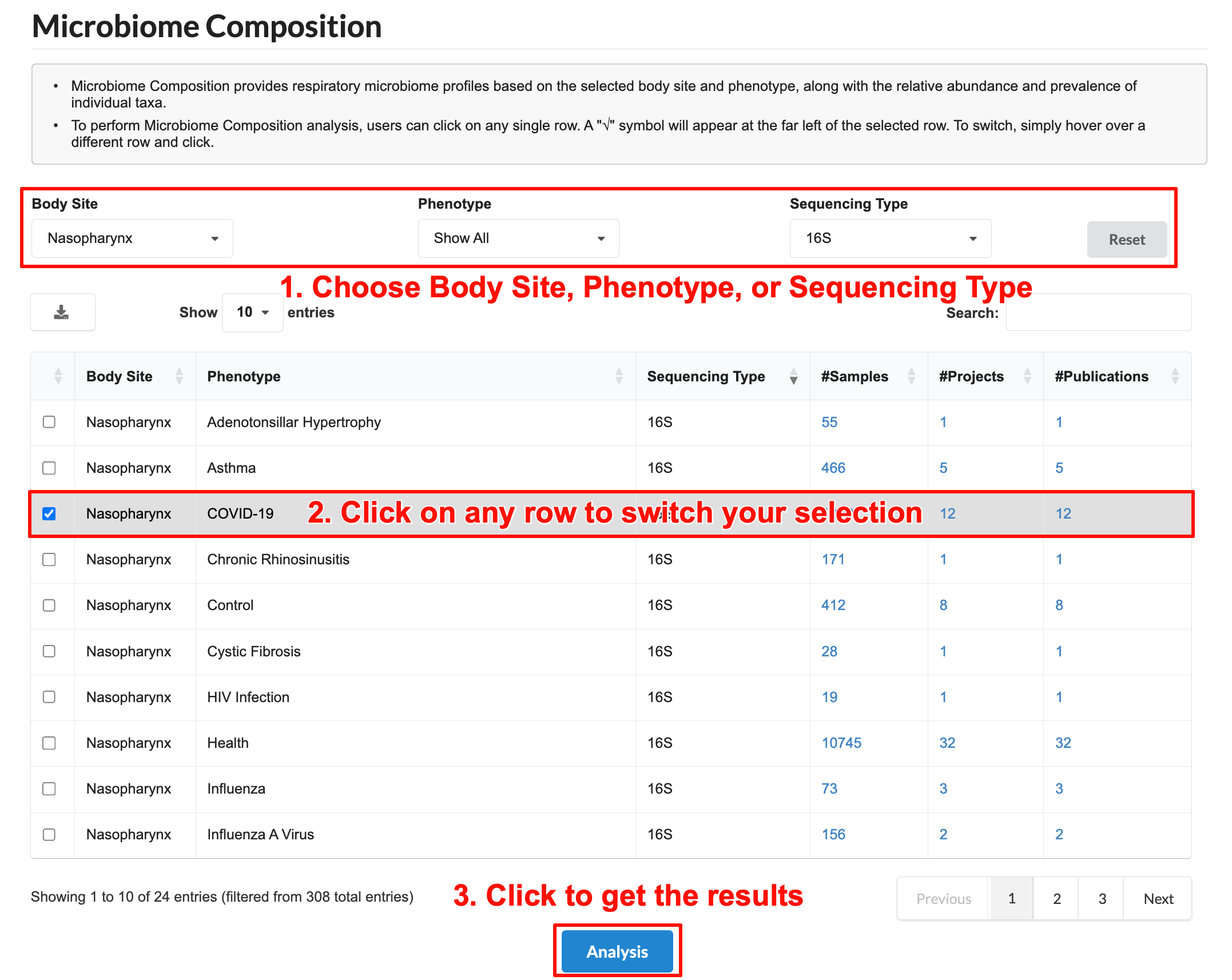
The Microbiome Composition allows users to analyze the microbial composition of a selected population of interest.
Follow these steps to perform the analysis:
Choose “Sample Site”, ”Phenotype“, or ”Sequencing Type" to select a population you are interested.
Click on any row to switch your selection. A "√" symbol will appear at the far left of the selected row, and the row will be highlighted in gray.
Click "Analysis" to get the results.
The results will appear on the page.
a) Dominant taxa:Displays the average relative abundance of the top 15 taxa across selected samples. Each column represents a sample, with hierarchical clustering performed using the Bray-Curtis distance matrix and the Ward.D2 method.
b) Average taxonomic composition: Shows the average microbial composition of all selected samples.
3.10 Sample Similarity search
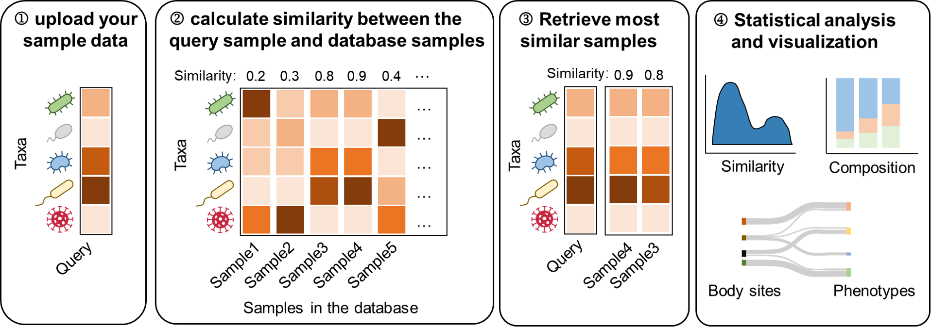
Sample Similarity Search identifies the most similar samples in the database based on a user's query. It provides integrated statistical analyses and visualizations using downloadable metadata and microbial composition data.
Given two microbiome samples A and B, the similarity between them is defined as:
We provide three distance metrics, which are widely used in microbiome studies.
Bray-Curtis
Jensen-Shannon Divergence (JSD)
Jaccard
Where:
A and B refer to two microbiome samples represented by their taxonomic profiles.
Follow these steps for analysis:
Upload Your Data: Provide the microbial composition data for a sample in CSV format. The first column should contain genus or species names, and the second column should list their relative abundances.
Sample Selection Filters: Select the appropriate taxonomic level for your sample. Then, choose whether to restrict the comparison to a specific sample site, whether to include healthy samples, whether to include infant samples
Distance Measure: Choose a method for calculating similarity.
Click "Run" to start the search. Results will typically be generated within 10–30 seconds.

The results will appear on the page.
a) Associated samples: display the 500 most similar samples along with their associated metadata.
b) Associated samples statistics: Visualizes the similarity metrics of the most similar samples and the distributions of sample sites and phenotypes. Users can adjust the similarity threshold to refine the displayed results.
c) Associated samples microbial composition: Displays microbial composition comparisons between the query sample and the most similar samples.
3.11 Cross-study Analysis
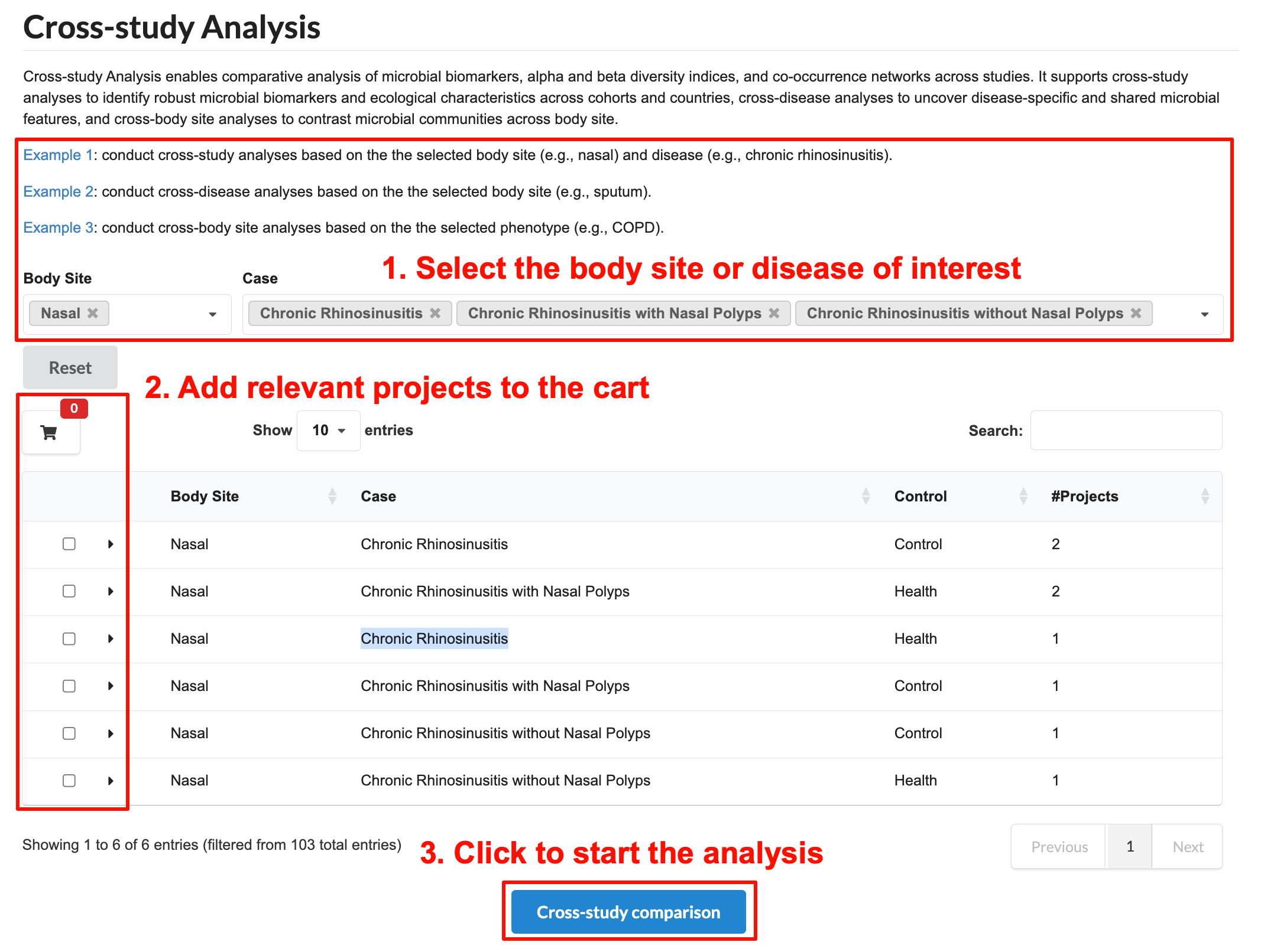
Cross-study Analysis Cross-study Analysis enables comparative analysis of microbial biomarkers, alpha and beta diversity indices, and co-occurrence networks across studies. It supports cross-study analyses to identify robust microbial biomarkers and ecological characteristics across cohorts and countries, cross-disease analyses to uncover disease-specific and shared microbial features, and cross-sample site analyses to contrast microbial communities across sample site.
Example 1: In ResMicroDb, a disease may span multiple projects. Cross-study comparisons can identify robust microbial characteristics across different studies associated with a specific disease (e.g., chronic rhinosinusitis) across multiple cohorts within a selected sample site.
Example 2: Similarly, a sample site may contain samples from multiple diseases. Cross-study comparisons can identify shared and unique microbial characteristics across different diseases within the same sample site (e.g., sputum). These characteristics may either be pan-disease characteristics (shared across diseases) or disease-specific ones (unique to a particular disease).
Example 3: Similarly, a phenotype may be related to multiple sample site. Cross-study comparisons can identify shared and unique microbial characteristics across different sample sites under the same condition (e.g., COPD).
Here we use Example 1 as an case to show the contents of this tool. Follow these steps to perform the analysis:
Select the sample site or disease of interest.
Add relevant projects to the cart (up to 30 projects). The red number indicates the total number of selected projects. Users can review project details before adding them.
Click "Cross-Study Comparison" to start the analysis.
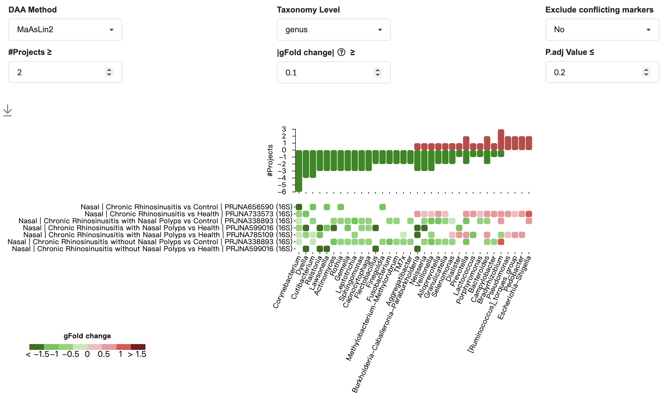
3.11.1 Marker
The heatmap below displays consistent and non-consistent disease-associated microbial markers across datasets for chronic rhinosinusitis in the nasal. Users can further customize the analysis by applying the following filters:
DAA Method: Select the differential abundance analysis method.
Taxonomy level: Select the taxonomy level (e.g., genus for 16S sequencing, or species for metagenomics and metatranscriptomics).
Exclude conflicting markers: Exclude/Include markers with inconsistent enrichment directions across different studies.
#Projects: Specify the number of projects that report the marker taxon as significantly different between cases and control groups.
|gFold change|: Filter by effect size.
P.adj Value: Apply a threshold based on the Benjamini-Hochberg adjusted p-value.
3.11.2 Diversity
Users can compare alpha diversity (Shannon index) between disease cases and healthy controls across different studies.
Users can compare beta diversity between disease cases and healthy controls across different studies.
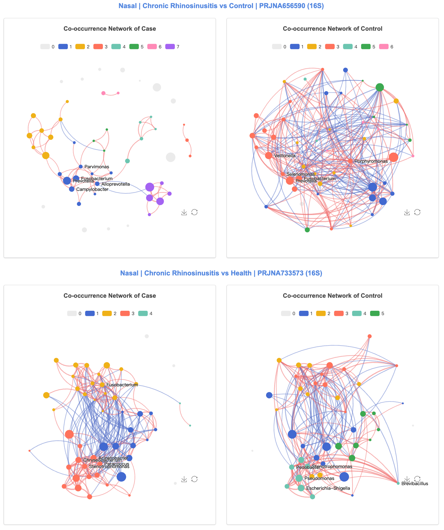
3.11.3 Network
Users can compare network between disease cases and healthy controls across different studies.
3.12 Statistics
The Statistics page provides an overview of the data in ResMicroDb, summarized across three dimensions: sample metadata, sequencing strategy, and publications.
3.13 Download
The Download page provides links to download the Metadata and Abundance tables for all samples included in ResMicroDb.